Okinawa Mangrove Temporal Analysis

Methodology: AlphaEarth Temporal Change Detection

1AlphaEarth Feature Extraction

Google AlphaEarth is a deep learning model trained on massive satellite imagery datasets that generates 65-dimensional feature vectors for each satellite image pixel. These embeddings capture complex environmental patterns including spectral characteristics, textural information, seasonal variations, and vegetation indicators that are not easily discernible through traditional spectral band analysis.

Data Acquisition:

• Source Multi-spectral satellite imagery (Sentinel-2, Landsat)
• Resolution 10-30 meters per pixel
• Temporal Annual composites from 2017-2023
• Output 65 floating-point values (A00-A64) per pixel

2Spatial Hotspot Identification

Most dynamic points are identified using a simple Euclidean distance metric in the 65-dimensional AlphaEarth embedding space. For each geographic point within the mangrove regions, we compute the vector distance between 2017 and 2023 feature vectors:

Hotspot Identification Process:

1. Point-wise temporal analysis: For each unique geographic coordinate, calculate the Euclidean distance between 2017 and 2023 feature vectors in the 65-dimensional space
2. Regional ranking: Within each mangrove region, rank all points by their change magnitude (Euclidean distance)
3. Hotspot selection: Top 3-5 points per region with highest Euclidean distances are marked as environmental hotspots (red star markers on maps)
4. Validation: Cross-reference with year-to-year consistency to avoid noise artifacts

These hotspots represent locations where the satellite-derived environmental signature has changed most significantly, potentially indicating:

• Ecosystem health degradation or recovery
• Hydrological pattern changes
• Anthropogenic impacts (development, restoration efforts)
• Climate-driven vegetation shifts
• Sediment dynamics or tidal pattern alterations

3Region Boundary Extraction

Mangrove region polygons were obtained directly from the Mangrove Global Initiative Japan (manglobal.or.jp) Google Maps database, which provides pre-digitized conservation zone boundaries for mangrove sites across Okinawa.

1. Access Google Maps Database: Navigate to the manglobal.or.jp Google Maps link containing pre-digitized mangrove conservation zones
2. Select Region of Interest: Identify the specific mangrove site (e.g., Hiyagon Wetland, Kin mangroves, Kokuba River)
3. Download KML:
   • Click the ⋮ menu icon on the Google Maps interface
   • Select "Export to KML/KMZ"
   • Choose KML format (not KMZ) for direct Python processing
   • Download saves polygon geometries with WGS84 coordinates
4. Multi-Region Processing: For sites with multiple conservation zones (e.g., Hiyagon Wetland with 11 sub-regions), the KML file contains all polygon boundaries as separate Placemark features
5. Coordinate Validation: Verify downloaded KML coordinates align with AlphaEarth pixel locations (WGS84 coordinate system standard ensures compatibility)

4Regional Statistics & Visualization

For each region and year, we compute:

• Average Feature Vector: Mean of all 65 dimensions across pixels within the region polygon
• Temporal Variance: Standard deviation of feature vectors across years
• Point Count: Number of satellite pixels assigned to the region (data coverage indicator)
• Change Metrics: Regional-level temporal change scores for comparative analysis

Interactive maps display:

• KML Region Boundaries: Color-coded polygons representing mangrove conservation zones
• Hotspot Markers: Red stars indicating locations with highest temporal change
• Satellite Basemap: High-resolution imagery for visual context
• Popup Statistics: Click markers/regions to view quantitative change metrics

Analysis Results & Visualizations

Hiyagon Wetland (比屋根湿地) Temporal Analysis

Comprehensive temporal change analysis of Hiyagon Wetland covering 2017-2024. The visualization below shows six analytical panels revealing environmental dynamics across 11 sub-regions.

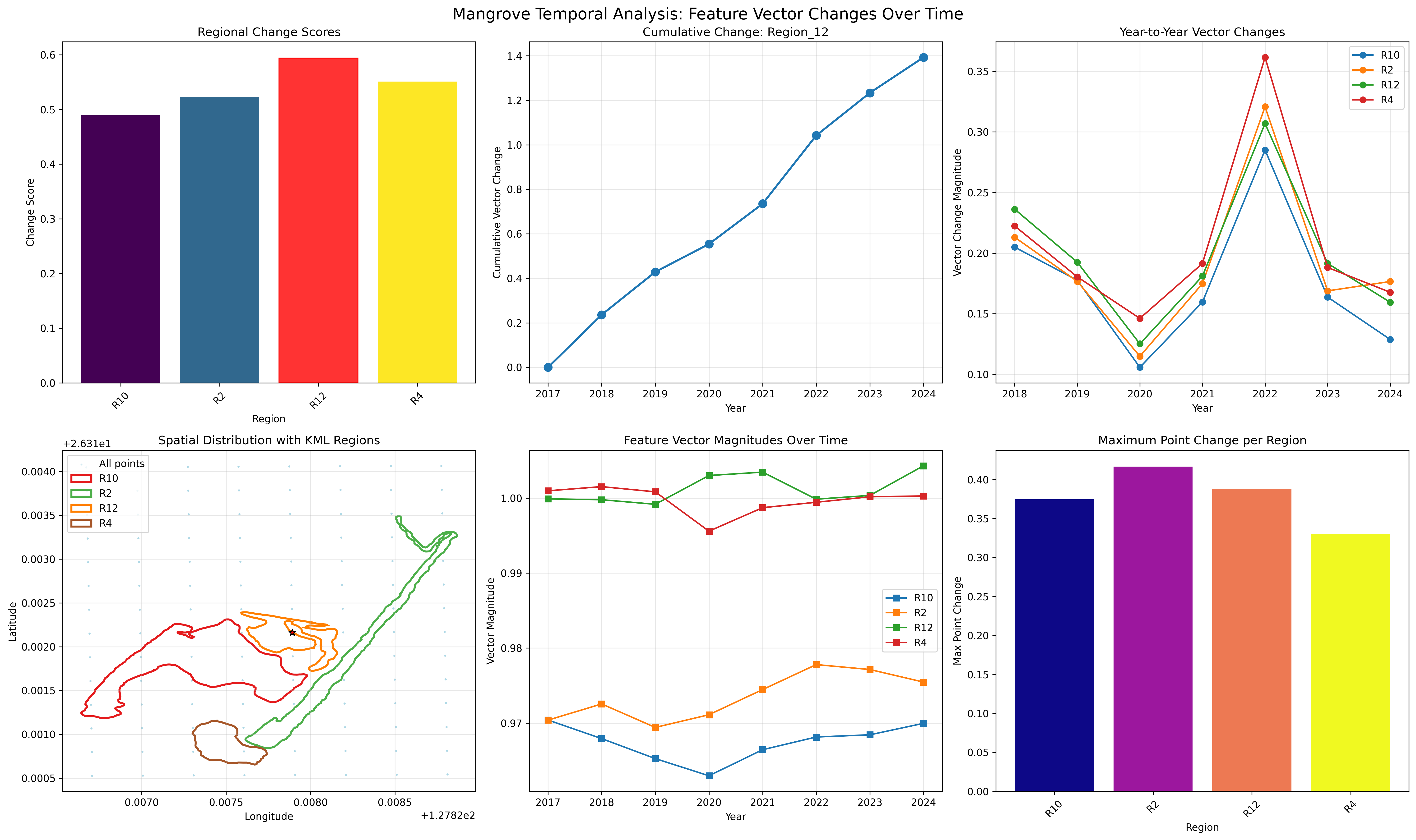
Panel Descriptions:
Top-left: Regional change scores | Top-center: Cumulative change in most dynamic region | Top-right: Year-to-year changes comparison
Bottom-left: Spatial distribution with KML boundaries | Bottom-center: Feature vector magnitudes over time | Bottom-right: Maximum point changes per region

Kin/Kokuba River Mangroves Analysis

Note: Kin mangrove analysis encountered coordinate system alignment issues between AlphaEarth pixel locations and KML region boundaries. Zero points were assigned to regions, indicating a potential datum mismatch. Further investigation required to ensure WGS84 coordinate consistency across datasets.